Outcome plots

Plot varpred object.

Usage

# S3 method for varpred
plot(
  x,
  ...,
  xlabs = NULL,
  ylabs = NULL,
  xtrans_fun = NULL,
  pos = 0.5,
  ci = TRUE,
  facet_scales = "fixed",
  facet_ncol = NULL
)

Arguments

x

varpred object.

...

for future implementations.

xlabs

x-axis label. If NULL, default, x.var is used.

ylabs

y-axis label. If NULL, default, the response label is used.

xtrans_fun

function to transform x values to the original or other scales. Useful when x was transformed prior to model fitting. See examples.

pos

spacing between labels of categorical variable on the plot.

ci

logical. If TRUE (default), the confidence intervals (indicating prediction or effect) are plotted, otherwise, only the central estimate is plotted.

facet_scales

should scales be fixed ("fixed", the default), free ("free"), or free in one dimension ("free_x", "free_y")?

facet_ncol

number of facet columns.

Value

a ggplot object.

See also

varpred

Examples

set.seed(4567)
N <- 100
x <- rnorm(N, 3, 5)
y <- 5 + 0.2*x + rnorm(N)
df <- data.frame(y = y, x = x)
m1 <- lm(y ~ x, df)
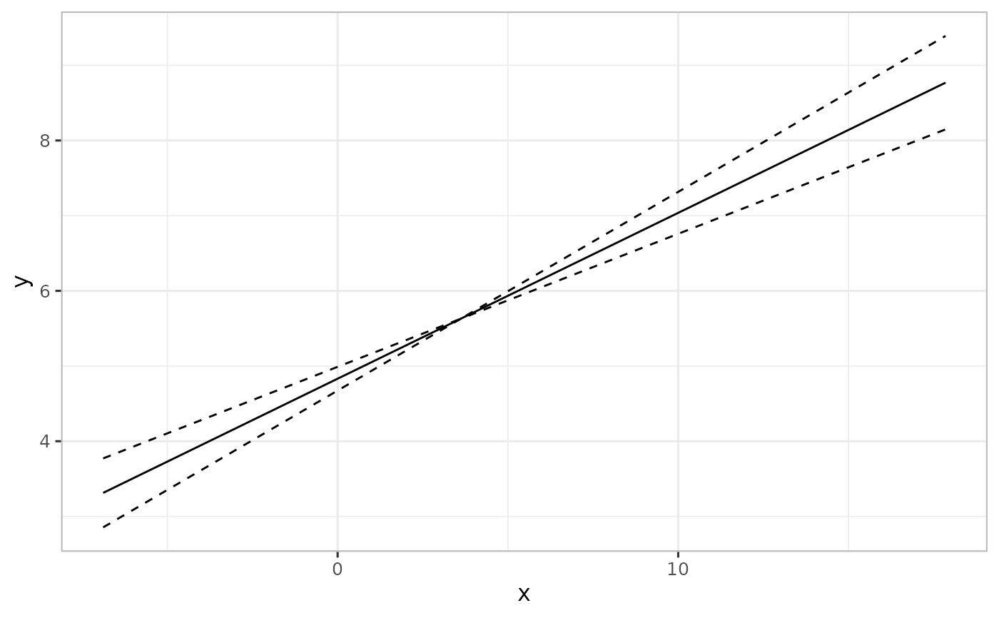
pred1 <- varpred(m1, "x", modelname="original")
plot(pred1)


## We can transform the predictor, fit the model and then
## back-transform the predictions in the plot
backtfun <- function(x, m, s) {
  x <- m + x*s
  return(x)
}
x_scaled <- scale(df$x)
m <- attr(x_scaled, "scaled:center")
s <- attr(x_scaled, "scaled:scale")
df$x <- as.vector(x_scaled)
m2 <- lm(y ~ x, df)
pred2 <- varpred(m2, "x", modelname="scaled")
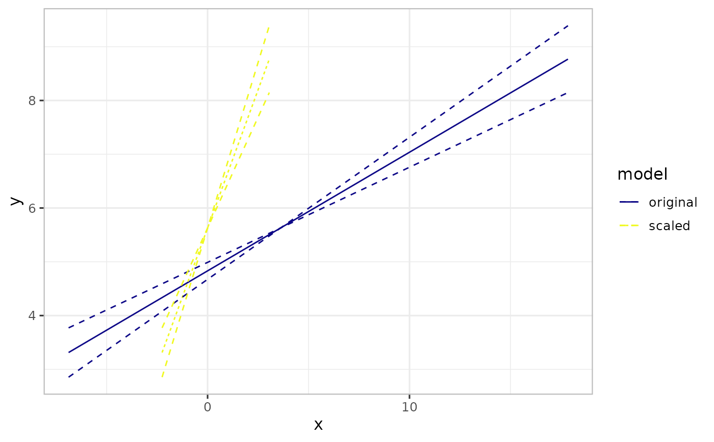
# Compare the predictions
combinevarpred(list(pred1, pred2), plotit=TRUE)


# Display focal predictor on the original scale
plot(pred2, xtrans_fun=function(x)backtfun(x, m=m, s=s))