Outcome plots

Bicko Cygu, Ben Bolker, Jonathan Dushoff

Motivation

The development of this package is motivated by the water, sanitation, and hygiene (WaSH) data in which we were interested in investigating the contribution of demographic and socio-economic factors to improved WaSH indicators among the slum dwellers in Nairobi, Kenya. We noticed that the predictions we generated using the existing packages consistently over- or under- estimated the observed proportions; and did not align well with the observed data points. In other words, what we call bias. There are several (challenges) reasons for this, including:

• the choice of the reference point
• uncertainty estimation – the choice of anchor for computing confidence intervals
• biases induced by non-linear averaging due to non-linear transformation in generalized linear models

Introduction

An outcome plot (often called effect or prediction plot), plots focal predictor on the x-axis and central estimate (predicted values) on the y-axis. The resulting plot provide a useful way to summarize the results from a regression model; and depend on how we deal with the above challenges.

Mean-based approach

In a model with non-focal predictors such as multivariate models, reference points (values chosen for non-focal predictors) can be chosen as the average of the non-focal linear predictor variables (columns of the model matrix corresponding to non-focal predictors) – we call this approach mean-based reference point and is currently not implemented in commonly used R software .

To illustrate this, we use datasets::mtcars dataset to fit two models: 1) one without interaction, and 2) one with interaction between predictors.

df <- datasets::mtcars

## No interaction model
mod1 <- lm(mpg ~ wt + disp + hp, df)

## Model with interaction
mod2 <- lm(mpg ~ wt + disp*hp, df)

If we consider wt as the focal predictor, then the remaining (disp and hp) are non-focal predictors. We use varpred, emmeans and Effects for comparison.

vapred package:

• bias.adjust="none": to generate mean-based
• All the three packages have different ways of generating values of focal predictor. For comparison, we use quantile and generate same focal values. Unless you want to compare with same values, this is not necessary.

library(varpred)
varpredtheme()

## generate values for focal predictor
steps <- 500
quant <- seq(0, 1, length.out=steps)
wt_values <- quantile(df$wt, quant, names=FALSE) |> unique()

## No interaction
vpred1 <- varpred(mod=mod1
    , focal_predictors="wt"
    , at=list(wt=wt_values)
    , bias.adjust="none"
    , modelname="varpred: no interaction"
)

## With interaction
vpred2 <- varpred(mod=mod2
    , focal_predictors="wt"
    , at=list(wt=wt_values)
    , bias.adjust="none"
    , modelname="varpred: with interaction"
)
names_use <- vpred2 |> head() |> colnames()

emmeans package:

library(emmeans)
em1 <- emmeans(mod1
    , specs=~wt
    , at=list(wt=wt_values)
)
em1 <- em1 |> data.frame()
em1$model <- "emmeans: no interaction"
em1$df <- NULL
colnames(em1) <- names_use

em2 <- emmeans(mod2
    , specs=~wt
    , at=list(wt=wt_values)
)
em2 <- em2 |> data.frame()
em2$model <- "emmeans: with interaction"
em2$df <- NULL
colnames(em2) <- names_use

Effects package:

library(effects)
#> Loading required package: carData
#> lattice theme set by effectsTheme()
#> See ?effectsTheme for details.
ef1 <- Effect("wt"
    , mod1
    , xlevels=list(wt=wt_values)
)
ef1 <- ef1 |> data.frame()
ef1$model <- "effects: no interaction"
colnames(ef1) <- names_use

ef2 <- Effect("wt"
    , mod2
    , xlevels=list(wt=wt_values)
)
ef2 <- ef2 |> data.frame()
ef2$model <- "effects: with interaction"
colnames(ef2) <- names_use

We can use varpred::combinevarpred to combine and compared the estimates:

• attrvpred: converts emmeans and effects objects to varpred
• varpred::getmeans: calculates marginal means of the estimates to compare with the data mean (mean of observed data)

The plot below compares the central estimates (trend lines), together with their mean (horizontal lines) with the data mean (mean of mpg) and the observed data (grey points).

library(ggplot2)
## Combine emmeans, effects and varpred objects
## and convert all to varpred objects for ploting
attrvpred <- function(obj) {
    if (!inherits(obj, "varpred")) {
        temp_obj <- list()
        obj$method <- gsub(".*\\: ", "", obj$model)
        obj$model <- gsub("\\:.*", "", obj$model)
        temp_obj$preds <- obj
        class(temp_obj) <- "varpred"
        return(temp_obj)
    } else {
        obj$preds$method <- gsub(".*\\: ", "", obj$preds$model)
        obj$preds$model <- gsub("\\:.*", "", obj$preds$model)
        return(obj)
    }
}
all_preds <- lapply(list(vpred1, vpred2, em1, em2, ef1, ef2), attrvpred)

## Compute marginal means: mean of the estimates
all_means <- lapply(all_preds, function(x){
    model <- x$preds$model[[1]]
    method <- x$preds$method[[1]]
    m <- getmeans(x, focal="wt", modelname=model)
    m$method <- method
    return(m)
})
all_means <- do.call("rbind", all_means)

## Data mean
df_mean <- data.frame(mpg=mean(df$mpg)
    , model="data mean"
)

## Plot all the estimates
p1 <- (combinevarpred(all_preds, plotit=TRUE, ci=FALSE)
    + geom_point(data=df, aes(x=wt, y=mpg), col="grey")
    + geom_hline(data=df_mean, aes(yintercept=mpg, color=model, linetype=model)) 
    + geom_hline(data=all_means, aes(yintercept=fit, colour=model, linetype=model))
    + facet_wrap(~method)
)
print(p1)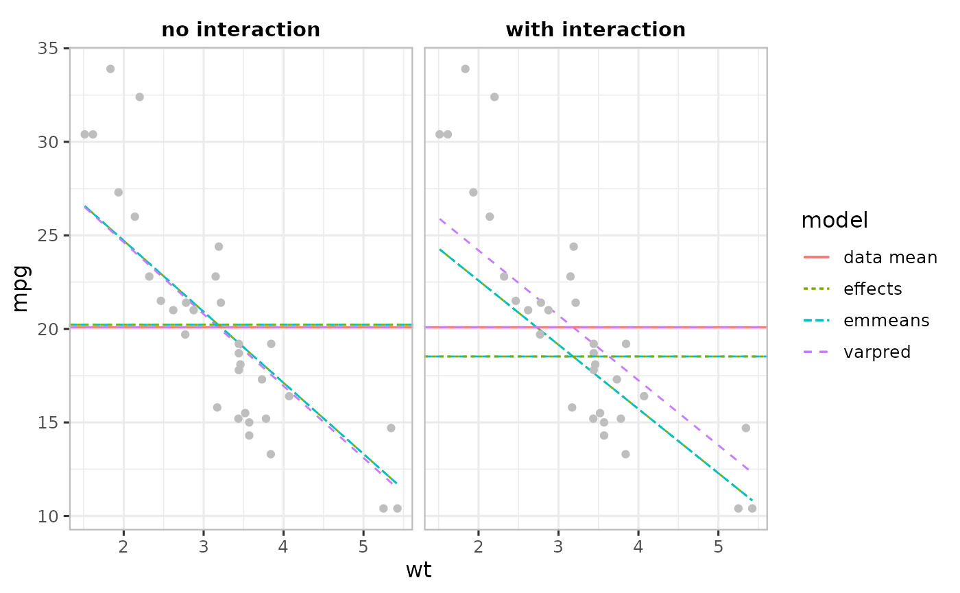

In the absence of interaction (left Figure), the three packages produce identical estimates and their respective averages closely match the data mean. However, in the presence of interactions, the estimates from emmeans and effects are identical but differ from varpred’s, which is very close to the data mean.

The packages emmeans and effects use the average of the input variables (mean of disp and hp) as the reference point as opposed to model-center approach varpred (average of the linear predictor variables). In the simple model (left Figure above) input variables are the same as the linear predictor variables, so all the three methods produce identical results. In the interaction model (right Figure above), there is an additional linear predictor variable (disp*hp). emmeans and effects first average the input variables to compute \(\mathrm{\bar{disp}}\star\mathrm{\bar{hp}}\) while varpred first calculates the corresponding vector of linear predictor values and then averages.

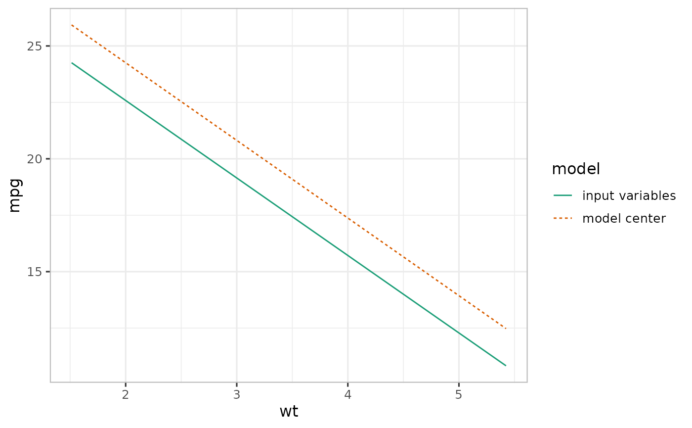
Input variable (emmeans-based) averaging with varpred (Experimental!)

We can also average input variables in varpred similar to emmeans and effects (input variable). Consider mod2 in the previous example, by setting input_vars=TRUE, we can generate predictions similar to the ones in em2.

## default varpred centering
vcenter <- varpred(mod2
    , "wt"
    , modelname="model center"
)

## varpred emmeans centering
emcenter <- varpred(mod2
    , "wt"
    , input_vars=TRUE
    , modelname="input variables"
)

all_preds_plots <- combinevarpred(list(vcenter, emcenter)
    , plot=TRUE
    , ci=FALSE
)
print(all_preds_plots
    + scale_color_brewer(palette = "Dark2")
)

Prediction and effect plots

The major distinction between the two lies on how we describe the uncertainty around the central estimates (trend lines in the previous Figures). The prediction plot captures all the sources of uncertainty, including that of intercept, non-focal predictors and random effects. On the other hand, effect plot takes into account the uncertainty associated with the focal predictor only. This way, we expect an effect plot to have narrower confidence intervals (CIs) then a prediction plot.

It is not easy to generate effect plots in emmeans and effects. A possible way to achieve this in emmeans and effects is to use a zeroed-out (see varpred::zero_vcov) covariance matrix, but this only works when the input variables are centered prior to model fitting, in case of numerical variables, and more complicated when the input variables are categorical.

In varpred, to generate effect plot, we set isolate=TRUE (default), otherwise (isolate=FALSE) prediction plot. We consider vpred1 generated above, which is an effect plot, and now generate a prediction for the same model (mod1).

## prediction-styled plot: set isolate=FALSE
vpred1_pred <- varpred(mod=mod1
    , focal_predictors="wt"
    , isolate=FALSE
    , at=list(wt=wt_values)
    , bias.adjust="none"
    , modelname="prediction"
)

## Rename vpred1
vpred1$preds$model <- "effects"

p2 <- (list(vpred1, vpred1_pred)
    |> combinevarpred(plotit=TRUE)
    + geom_hline(data=df_mean, aes(yintercept=mpg, color=model, linetype=model)) 
    + geom_vline(xintercept=mean(wt_values), lty=2)
)
print(p2)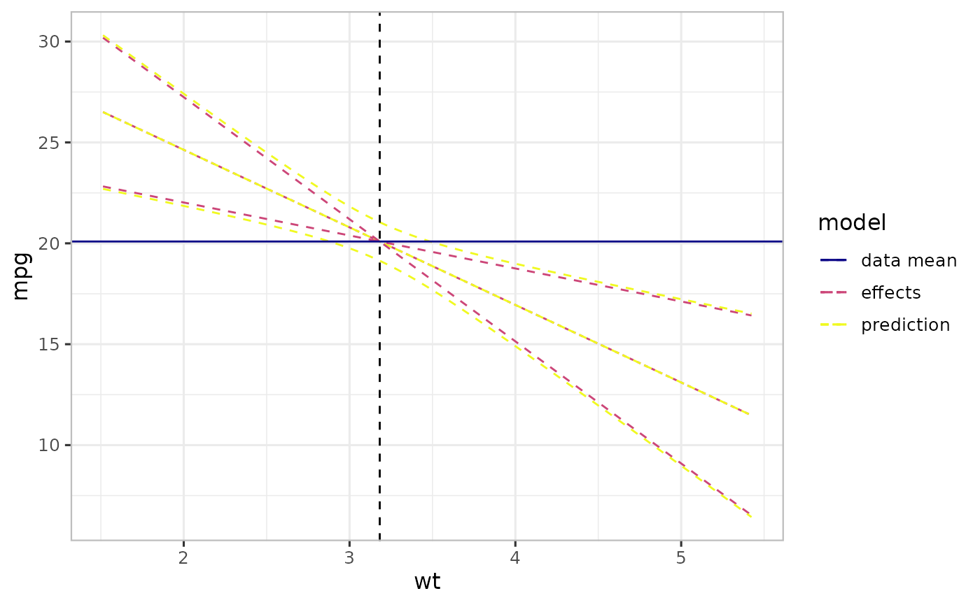

The Figure above shows a prediction (-styled) and an effect (-styled) plot. The horizontal line is the mean of the data (mean of mpg) while the vertical one is the mean of the focal predictor (wt) – we call this center point. The wider curves correspond to the conventional prediction curves (prediction-styled plot), while the narrower curves crossing at the center point. For a simple linear model, effect-styled curves cross at the center point. In other words, effects-styled plots provide a way to generate effects indicating uncertainty due only to changes in the focal predictor.

Anchor

To generate an effect-styled plot, we need a value of the focal predictor to compute CIs. We call this an anchor. The anchor choice does not affect the central estimate, nor prediction-style plot. The default value is the center point of the linear predictor variables corresponding to the focal predictor. For example, in the previous Figure, mean of wt is used as the default choice.

This is particularly important when we want to show an effect at a particular value of the focal predictor other than its mean (center point). For example, at \(0\), minimum of the focal predictor, etc. To implement this in varpred, set the anchor value using isolate.value and isolate must be TRUE.

## Min of wt
anchor0 <- varpred(mod1
    , "wt"
    , isolate=TRUE
    , isolate.value=min(df$wt) # min anchor
    , modelname="min"
)

## mean-anchored (default)
anchor0.5 <- varpred(mod1
    , "wt"
    , isolate=TRUE
    , modelname="mean"
)

p3 <- (list(anchor0, anchor0.5)
    |> combinevarpred() # No plot
    |> plot()
    + labs(colour="Anchor", linetype="Anchor")
)
print(p3)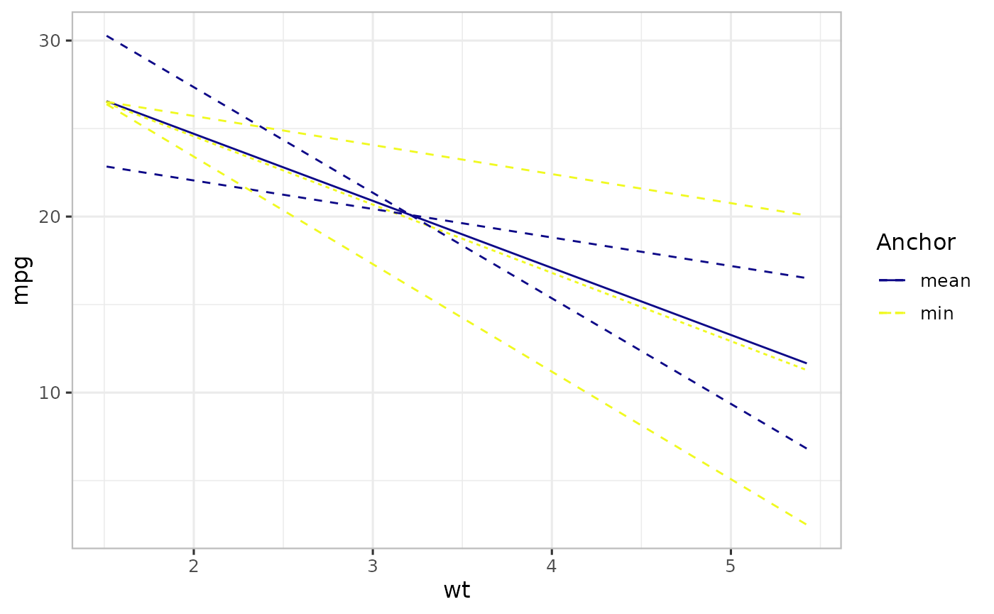

Observed-value approach

For a linear model, the averaging is done on the linear scale, i.e., linear averaging. As a result, the model-center estimates (made using the mean-based approach) are unbiased. However, in a model with non-linear link function, this is not usually true. When averaging is done on a separate link scale, the mean of the estimates is not the same as the estimate at the mean point. This leads to bias: in this case a systematic difference between the values seen on average for a given value of the focal predictor and the value predicted by the mean-based approach. An alternative to the mean-based reference point is the observed-value-based approach, which involves computing the prediction over the population of non-focal predictors and then averaging across the values of the focal predictor.

To implement observed-value-based in varpred, we set bias.adjust="observed".

## mean-based: set bias.adjust="none"
vpred_mean <- varpred(mod1, "wt", bias.adjust="none", modelname="mean-based")

## observed-value: set bias.adjust="observed"
vpred_observed <- varpred(mod1, "wt", bias.adjust="observed", modelname="observed-value")

p4 <- (list(vpred_mean, vpred_observed)
    |> combinevarpred(plotit=TRUE)
    + labs(colour="Approach", linetype="Approach")
)
print(p4)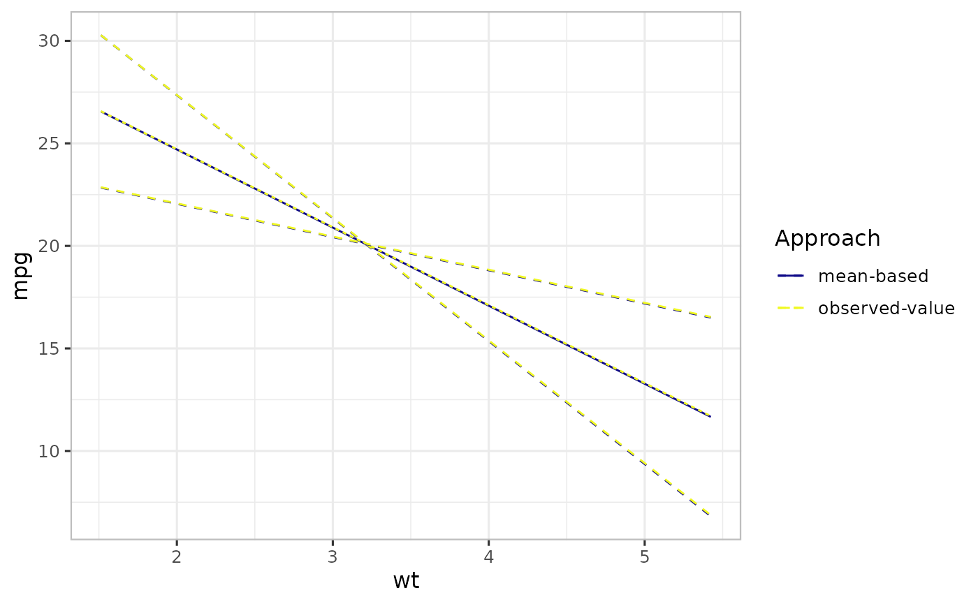

Bias correction

In a simple linear model, such as mod1, all the averaging is done on the linear scale, hence there is not effect of non-linear averaging. Consequently, the estimates are similar, as shown in the previous Figure. However, in a model with non-linear link function such as generalized models, this is not usually true. To demonstrate this, we simulate a binary outcome with two predictors as shown below.

set.seed(911)
# Simulate binary outcome data with two predictors
steps <- 500
N <- 1000
b0 <- 2
b_age <- -1.5
b_income <- 1.8
min_age <- 18
age <- min_age + rnorm(N, 0, 1)
min_income <- 15
income <- min_income + rnorm(N, 0, 1)
eta <- b0 + age*b_age + income*b_income
status <- rbinom(N, 1, plogis(eta))
df <- data.frame(status, age, income)

# Fit model
mod <- glm(status ~ age + income, df, family=binomial())

# Effect plots
## Mean-based
ef_mean <- varpred(mod, "age", steps=steps, bias.adjust="none", modelname="mean-based")
## Observed-value-based
ef_observed <- varpred(mod, "age", steps=steps, bias.adjust="observed", modelname="observed-value")

We write a simple function to add binned observations, i.e., proportion of observed outcomes falling within particular bin:

## Generate binned observations
### mod: data.frame or mod object (df preferable)
binfun <- function(mod, focal, bins=50, groups=NULL) {
    require(dplyr, quietly=TRUE, warn.conflicts=FALSE)
    if (!is.null(groups)) {
        bins_all <- c(groups, "bin")
    } else {
        bins_all <- "bin"
    }
    if (!inherits(mod, "data.frame")) {
        mf <- model.frame(mod)
    } else {
        mf <- mod
    }
    N <- NROW(mf)
    check_df <- (mf
        |> arrange_at(focal)
        |> mutate(bin=ceiling(row_number()*bins/N))
        |> group_by_at(bins_all)
        |> summarise_all(mean)
        |> mutate(model="binned")
    )
    return(check_df)
}

binned_df <- binfun(mod, "age", bins=50)
head(binned_df)
#> # A tibble: 6 × 5
#>     bin status   age income model 
#>   <dbl>  <dbl> <dbl>  <dbl> <chr> 
#> 1     1   1     15.6   15.0 binned
#> 2     2   1     16.1   15.4 binned
#> 3     3   0.95  16.4   14.8 binned
#> 4     4   1     16.6   15.1 binned
#> 5     5   1     16.7   15.1 binned
#> 6     6   0.9   16.8   15.0 binned

We combine the varpred objects and add the observed values (binned).

## Combine all the effect estimates
ef <- (list(ef_mean, ef_observed)
    |> combinevarpred(plotit=TRUE)
    + geom_point(data=binned_df, aes(x=age, y=status), colour="grey")
)
plot(ef)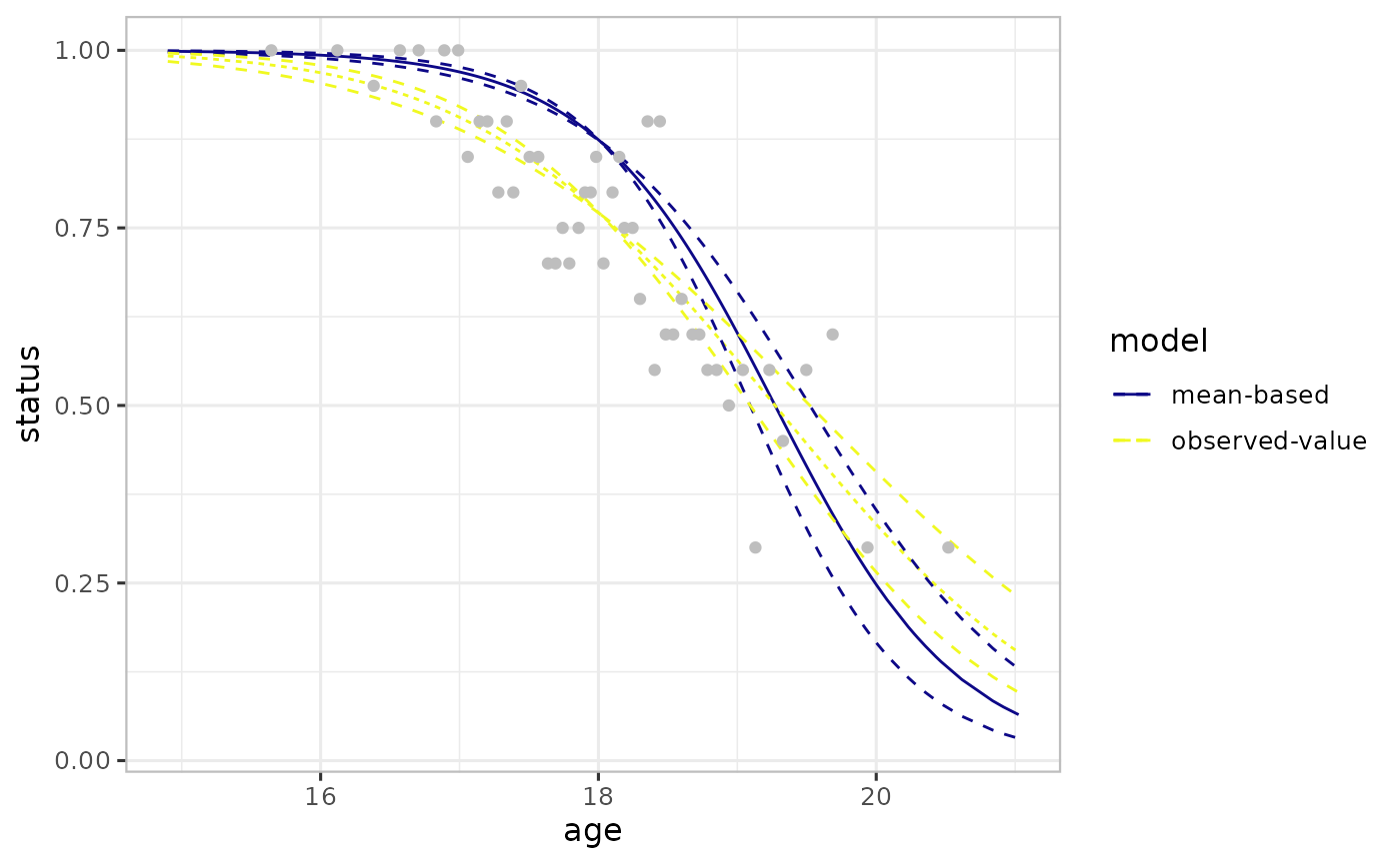

The difference in mean-based and observed-value-based is due to the bias induced by the non-focal predictor and the non-linear averaging in the logistic model. The mean-based approach is affected by the non-linear averaging. As a result, the observed-value approach estimates are more aligned to the observed data than the mean-based approach, see previous Figure.